Housing Analysis with MARS (earth)

1 Setup

# 1. Ensure CRAN mirror in non-interactive renders
repos <- getOption("repos")
if (is.null(repos) || is.na(repos["CRAN"]) || repos["CRAN"] == "@CRAN@") {
  options(repos = c(CRAN = "https://cloud.r-project.org"))
}

# 2) Declare the packages you use directly
required_pkgs <- c("readxl", "writexl", "dplyr", "ggplot2", "earth", "plotmo", "janitor")

# 3) Resolve all recursive dependencies (so 'cellranger' and friends are included)
ap <- utils::available.packages()  # uses the CRAN mirror set above
deps <- tools::package_dependencies(required_pkgs, db = ap, recursive = TRUE)
deps <- unique(unlist(deps, use.names = FALSE))
need <- setdiff(c(required_pkgs, deps), rownames(installed.packages()))

if (length(need)) {
  install.packages(need)
}

# 4) Load only the top-level packages you actually use
invisible(lapply(required_pkgs, library, character.only = TRUE))

options(dplyr.summarise.inform = FALSE)
set.seed(1234)

## Data: Excel Input (and a sample generator)

#This analysis expects an Excel file at `data/housing_sample.xlsx`. If it is missing, we generate a realistic sample so you can run end-to-end immediately.

excel_path <- file.path("data", "housing_sample.xlsx")
if (!file.exists(excel_path)) {
  n <- 300L
  neighborhoods <- c("Pacifica", "Burlingame", "San Mateo", "Daly City")
  conditions   <- c("Poor", "Fair", "Good", "Excellent")
  
  df <- tibble::tibble(
    id          = 1:n,
    sqft        = pmax(round(rnorm(n, mean = 1600, sd = 400)), 400),
    beds        = pmax(round(rnorm(n, mean = 3, sd = 1)), 1),
    baths       = pmax(round(rnorm(n, mean = 2, sd = 0.7), 1), 1),
    lot_size    = pmax(round(rnorm(n, mean = 4500, sd = 1500)), 800),
    year_built  = sample(1940:2022, n, replace = TRUE),
    neighborhood= sample(neighborhoods, n, replace = TRUE, prob = c(.3,.25,.25,.2)),
    condition   = sample(conditions,   n, replace = TRUE, prob = c(.1,.25,.45,.2)),
    ocean_view  = rbinom(n, 1, prob = 0.15),
    dist_bart_km= round(rexp(n, rate = 1/6) + runif(n, 0, 2), 2)
  ) |>
  dplyr::mutate(
    # Construct a price with nonlinearities and interactions
    age         = 2025 - year_built,
    neigh_bump  = dplyr::case_when(
                     neighborhood == "Burlingame" ~ 180000,
                     neighborhood == "San Mateo"  ~ 120000,
                     neighborhood == "Pacifica"   ~  90000,
                     TRUE ~ 70000
                   ),
    cond_bump   = dplyr::case_when(
                     condition == "Excellent" ~ 120000,
                     condition == "Good"      ~  60000,
                     condition == "Fair"      ~  20000,
                     TRUE ~ 0
                   ),
    price_noise = rnorm(n, 0, 60000),
    sale_price  = 200000 + 280*sqrt(pmax(sqft, 300)) + 35*lot_size +
                  45000*beds + 50000*baths + 85000*ocean_view +
                  neigh_bump + cond_bump - 1500*age - 8000*dist_bart_km +
                  0.02*(pmax(sqft - 2200, 0))^1.4 + price_noise
  ) |>
  dplyr::select(-price_noise, -neigh_bump, -cond_bump) |>
  dplyr::mutate(sale_price = round(pmax(sale_price, 120000)))
  
  writexl::write_xlsx(df, excel_path)
}

1.1 Read & clean

housing_raw <- readxl::read_excel(excel_path)
housing <- housing_raw |>
  janitor::clean_names() |>
  dplyr::mutate(
    neighborhood = as.factor(neighborhood),
    condition    = as.factor(condition),
    ocean_view   = factor(ocean_view, levels = c(0,1), labels = c("No","Yes"))
  ) |>
  as.data.frame()

str(housing)

'data.frame':   300 obs. of  12 variables:
 $ id          : num  1 2 3 4 5 6 7 8 9 10 ...
 $ sqft        : num  1117 1711 2034 662 1772 ...
 $ beds        : num  2 2 3 4 3 2 2 5 3 4 ...
 $ baths       : num  2.2 2.4 1 2.5 2 1.9 2.8 3 1.2 2.7 ...
 $ lot_size    : num  800 3860 2269 5383 3836 ...
 $ year_built  : num  1961 2018 1987 1943 1973 ...
 $ neighborhood: Factor w/ 4 levels "Burlingame","Daly City",..: 2 3 1 1 3 1 1 2 3 1 ...
 $ condition   : Factor w/ 4 levels "Excellent","Fair",..: 2 3 3 2 3 2 2 3 3 3 ...
 $ ocean_view  : Factor w/ 2 levels "No","Yes": 1 1 1 1 1 1 1 1 1 1 ...
 $ dist_bart_km: num  2.61 4.37 2.51 4.8 6.96 ...
 $ age         : num  64 7 38 82 52 23 60 65 33 9 ...
 $ sale_price  : num  503255 697862 693541 681355 505115 ...

summary(housing$sale_price)

   Min. 1st Qu.  Median    Mean 3rd Qu.    Max. 
 262434  564941  668166  659502  738206 1067306 

2 Exploratory plots

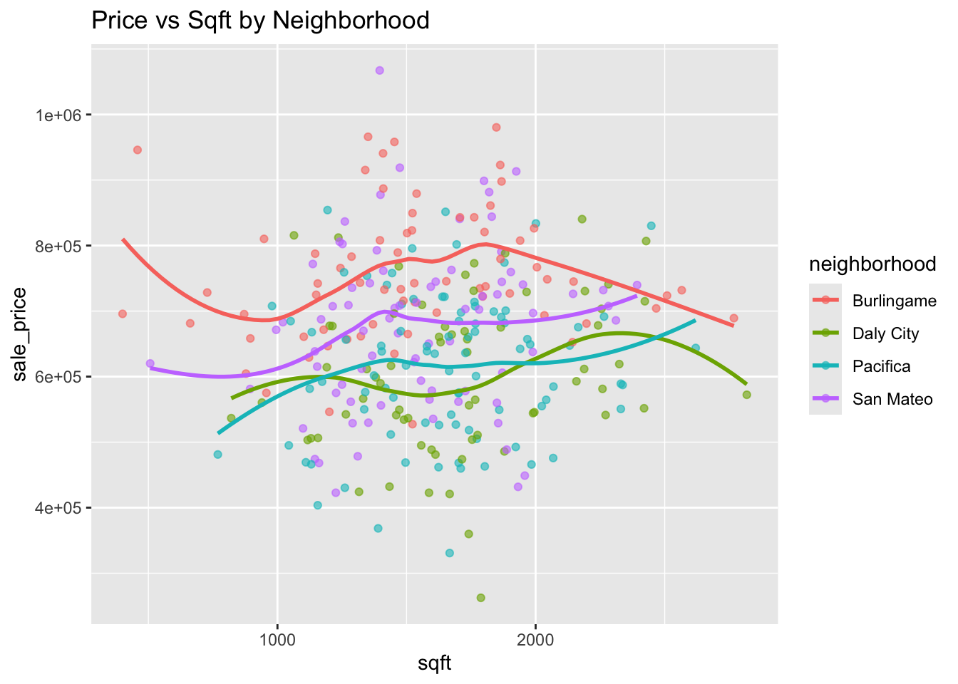
library(ggplot2)
ggplot(housing, aes(sqft, sale_price, color = neighborhood)) +
  geom_point(alpha = 0.6) +
  geom_smooth(method = "loess", se = FALSE) +
  labs(title = "Price vs Sqft by Neighborhood")

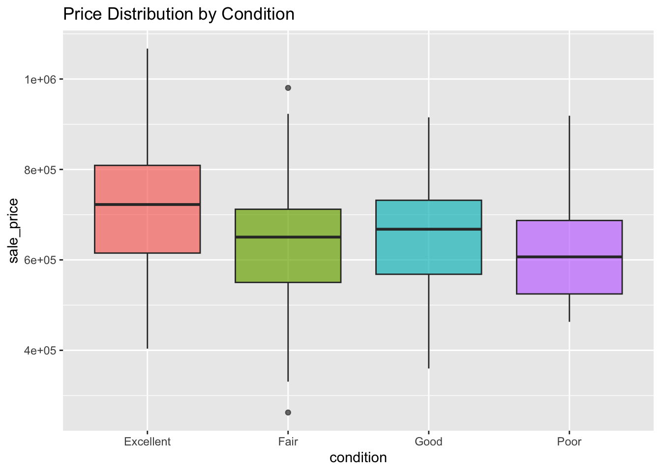
ggplot(housing, aes(condition, sale_price, fill = condition)) +
  geom_boxplot(alpha = 0.7) +
  labs(title = "Price Distribution by Condition") +
  theme(legend.position = "none")

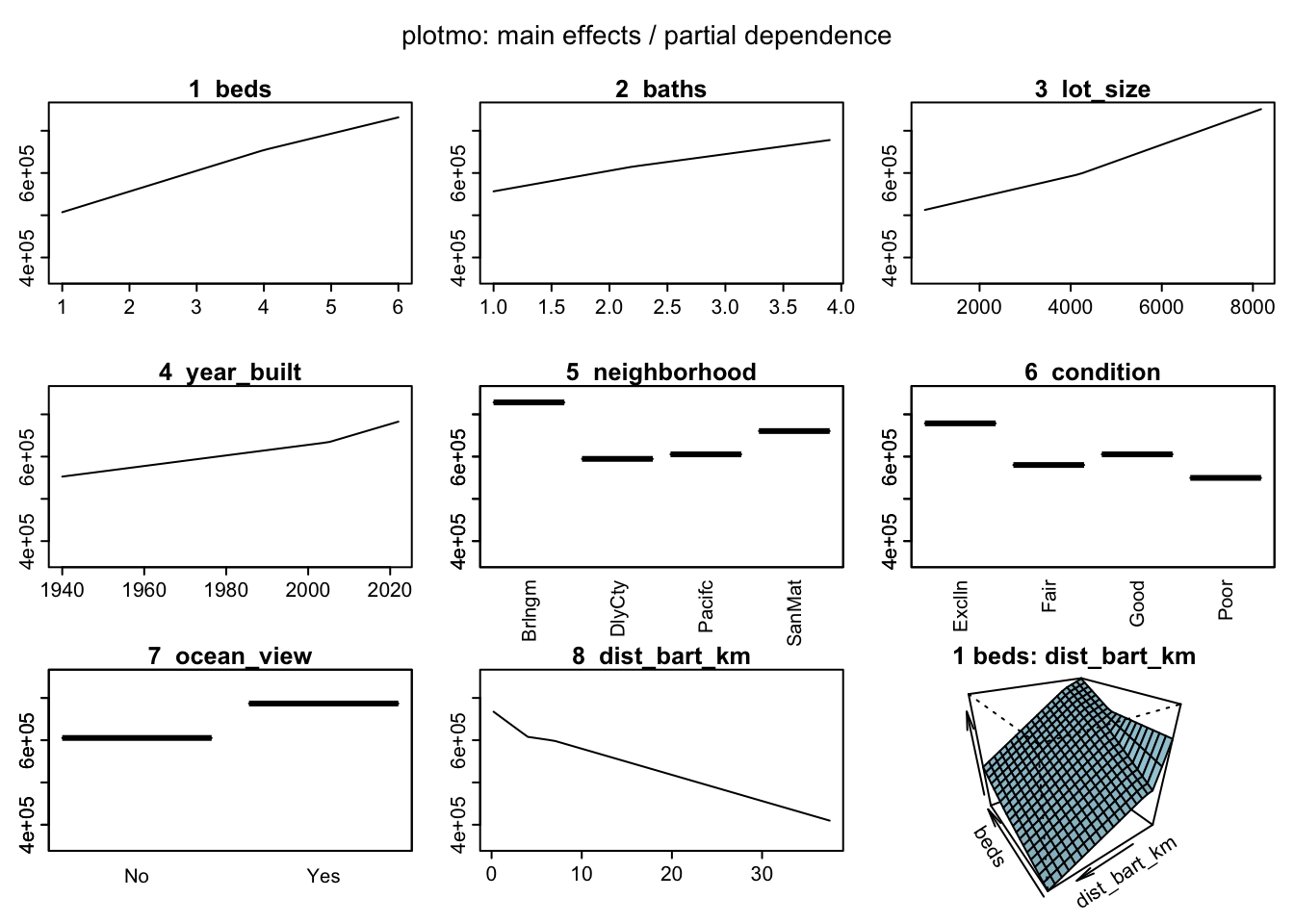
3 Fit MARS (earth)

We fit a MARS model with 10-fold CV model selection.

form <- sale_price ~ sqft + beds + baths + lot_size + year_built +
                    neighborhood + condition + ocean_view + dist_bart_km

mars_fit <- earth::earth(
  formula  = form,
  data     = housing,
  degree   = 2,          # allow interactions
  nprune   = 50,         # upper bound on terms
  pmethod  = "cv",       # prune by cross-validation
  nfold=10,
  ncros=30,
  varmod.method = "earth"
)

3.1 Model summary and ANOVA

summary(mars_fit)

Call: earth(formula=form, data=housing, pmethod="cv", degree=2, nprune=50,
            nfold=10, ncross=30, varmod.method="earth")

                              coefficients
(Intercept)                      873336.44
neighborhoodDaly City           -133600.14
neighborhoodPacifica            -122924.17
neighborhoodSan Mateo            -67777.37
conditionFair                    -98546.91
conditionGood                    -73386.66
conditionPoor                   -129080.67
ocean_viewYes                     81542.21
h(4-beds)                        -49616.13
h(beds-4)                         38633.34
h(2.2-baths)                     -48758.00
h(baths-2.2)                      37021.23
h(4196-lot_size)                    -24.94
h(lot_size-4196)                     38.61
h(2005-year_built)                -1252.64
h(year_built-2005)                 2860.20
h(6.95-dist_bart_km)               3779.82
h(dist_bart_km-6.95)              -6841.21
h(4-beds) * h(dist_bart_km-4)       651.74
h(4-beds) * h(4-dist_bart_km)     11947.69

Selected 20 of 20 terms, and 12 of 13 predictors (pmethod="cv") (nprune=50)
Termination condition: Reached nk 27
Importance: lot_size, dist_bart_km, beds, year_built, ocean_viewYes, ...
Number of terms at each degree of interaction: 1 17 2
GRSq 0.7604635  RSq 0.8305252  mean.oof.RSq 0.7615264 (sd 0.0812)

pmethod="backward" would have selected:
    18 terms 12 preds,  GRSq 0.7668059  RSq 0.8283871  mean.oof.RSq 0.7607295

varmod: method "earth"    min.sd 6.11e+03    iter.rsq 0.000

stddev of predictions:
            coefficients iter.stderr iter.stderr%
(Intercept)      61074.1     2322.63            4

                              mean   smallest    largest   ratio
95% prediction interval   239406.1   239406.1   239406.1       1

                                         68%    80%    90%    95% 
response values in prediction interval   72     86     95     98  

anova(mars_fit)

NULL

3.2 Variable importance (earth::evimp)

ev_obj <- try(earth::evimp(mars_fit), silent = TRUE)

if (inherits(ev_obj, "try-error") || is.null(ev_obj) || length(ev_obj) == 0L) {
  cat("No variable-importance information is available for this model.\n")
} else {
  # 1) Force a strictly rectangular object
  ev_mat <- try(as.matrix(ev_obj), silent = TRUE)

  if (inherits(ev_mat, "try-error") || is.null(dim(ev_mat)) || nrow(ev_mat) == 0L) {
    cat("Variable-importance object is empty or non-rectangular; printing raw output instead.\n")
    print(ev_obj)
  } else {
    # 2) Keep only columns that actually exist
    want_cols <- c("nsubsets", "gcv", "rss", "rsq")
    keep_cols <- intersect(want_cols, colnames(ev_mat))
    # Always include 'term' constructed from rownames
    ev_df <- data.frame(
      term = rownames(ev_mat),
      if (length(keep_cols)) ev_mat[, keep_cols, drop = FALSE],
      check.names = FALSE,
      row.names = NULL
    )

    # 3) Order (if any numeric columns present)
    rank_cols <- intersect(c("gcv", "rss", "rsq", "nsubsets"), names(ev_df))
    if (length(rank_cols)) {
      ev_df <- ev_df[order(ev_df[[rank_cols[1]]], decreasing = TRUE), , drop = FALSE]
    }

    # Show up to 20 rows without risky indexing
    n_show <- min(20L, nrow(ev_df))

    # 4) Table with graceful fallback (never abort render)
    tryCatch(
      {
        knitr::kable(
          if (n_show > 0L) ev_df[seq_len(n_show), , drop = FALSE] else ev_df,
          digits = 3,
          caption = "earth::evimp variable importance (top terms)"
        )
      },
      error = function(e) {
        cat("kable() could not format the importance table; showing a plain print() instead.\n")
        print(if (n_show > 0L) ev_df[seq_len(n_show), , drop = FALSE] else ev_df)
      }
    )
  }
}

earth::evimp variable importance (top terms)

term	nsubsets	gcv	rss
lot_size	19	100.000	100.000
dist_bart_km	18	86.483	86.775
beds	17	79.631	79.759
year_built	16	71.685	71.923
ocean_viewYes	14	62.744	62.748
neighborhoodDaly City	14	59.817	60.129
neighborhoodPacifica	14	59.817	60.129
baths	12	47.280	48.271
neighborhoodSan Mateo	10	40.553	41.606
conditionFair	9	35.422	36.691
conditionGood	9	35.422	36.691
conditionPoor	9	35.422	36.691

4 Partial-dependence style plots (plotmo)

par(mfrow = c(2,2))
plotmo::plotmo(mars_fit, caption = "plotmo: main effects / partial dependence")

 plotmo grid:    sqft beds baths lot_size year_built neighborhood condition
               1597.5    3     2     4403       1982     Pacifica      Good
 ocean_view dist_bart_km
         No        4.855

par(mfrow = c(1,1))

5 Predictions & residual diagnostics

housing$pred  <- predict(mars_fit, newdata = housing)
housing$resid <- housing$sale_price - housing$pred

library(dplyr)
rmse <- sqrt(mean(housing$resid^2))
mae  <- mean(abs(housing$resid))
c(RMSE = round(rmse, 1), MAE = round(mae, 1))

   RMSE     MAE 
52628.6 41825.9 

ggplot(housing, aes(pred, sale_price)) +
  geom_point(alpha = 0.6) +
  geom_abline(slope = 1, intercept = 0, linetype = 2) +
  labs(title = "Predicted vs Actual", x = "Predicted", y = "Actual")

ggplot(housing, aes(pred, resid)) +
  geom_hline(yintercept = 0, linetype = 2) +
  geom_point(alpha = 0.6) +
  labs(title = "Residuals vs Fitted", x = "Fitted (Pred)", y = "Residuals")

ggplot(housing, aes(resid)) +
  geom_histogram(bins = 30) +
  labs(title = "Residual Histogram")

6 Notes for your own Excel file

To use your own data, replace data/housing_sample.xlsx with your file, and adjust the formula in form to reflect your column names.